FEOS Code Package

The FEOS (Frankfurt equation-of-state) package (formerly known under the name MPQeos-JWGU [1]) for the EOS generation and visualization of hot and dense matter is a computer code - written in C/C++ - which consists of three parts:

• the FEOS library which contains all the routines for the calculation of the EOS and which provides a C/C++ as well as a Fortran interface for this purpose,
• the FEOS table generation tool which accesses the FEOS library in order to generate EOS table files (e.g. in the SESAME [2] database format),
• and the SHOWEOS table visualization tool which was developed to plot isotherms, isochores, isentropes, and Hugoniot curves.

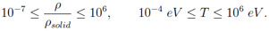
The underlying code of the FEOS package, MPQeos [3], is based on the EOS model QEOS [4] and was produced by A. Kemp et al. at the Max-Planck Institute for Quantum Optics in Garching at Munich. The motivation for the further development was a part of my diploma thesis which was devoted to an investigation of metastable states (superheated liquids) in volumetrically heated matter (thin foils) [5]. The original MPQeos was in some parts not adequate enough for this investigation. Especially, I needed the EOS for mixtures of elements (fused silica or silicon dioxide) and a better description of the liquid-vapor coexistence region. With the applied improvements the new code can and will be now also used for other applications at GSI in Darmstadt, especially for radiation-hydrodynamic simulations.

At this point I would like to thank Dr Anna Tauschwitz, Prof Dr Joachim Maruhn (both Goethe University Frankfurt am Main & GSI Darmstadt), Prof Dr Igor Iosilevskiy (Joint Institute for High Temperatures Moscow & GSI Darmstadt), and Prof. Dr. Mikhail Basko (Institute for Theoretical and Experimental Physics Moscow & GSI Darmstadt) for very helpful and constructive discussions during the development of FEOS.

Description of the QEOS model and MPQeos

The calculated thermodynamic quantities are: pressure, specific internal energy, specific Helmholtz free energy, specific entropy, and charge state. The calculations can be done with or without a Maxwell construction which eliminates the van-der-Waals loops in the liquid-vapor coexistence region.

The input variables for the EOS calculation of one single element are: atomic number, atomic weight, reference conditions (density and temperature where pressure and energy are set to zero), and the bulk modulus at the reference conditions. The MPQeos code was designed to calculate the EOS in the following range:

In the QEOS model all thermodynamic quantities are derived from the Helmholtz free energy which is composed of three contributions, the (uncorrected) electronic part, the ionic part and the so-called bonding correction:

For the calculation of the electronic contribution the simple Thomas-Fermi (TF) model [6] is used. In this model the electrons are described as a Fermi gas in the self-consistent electrostatic field of the atom. Matter is segmented into spherical cells for which the equilibrium electron distribution is calculated by solving the TF equation. Calculations with the simple TF model are faster than with advanced TF theories because all thermodynamical quantities scale with the atomic number and therefore must be calculated only once for e.g. hydrogen. The main two disadvantages of the simple TF model are the overestimation of critical pressure and critical temperature and the overall overestimation of pressures near normal conditions. The reason for this failures is the negligence of attractive (bonding) forces between neutral atoms in the simple TF theory.

The so-called bonding correction [7], the recalibration scheme of QEOS, is added to the total EOS (or the electronic part) in order to improve the previously mentioned failures of the electronic contribution. It adjusts the EOS to zero pressure / energy and to the defined bulk modulus (and thereby sound speed) at the reference conditions.

The ionic contribution is calculated by the Cowan model, a semi-empirical model which interpolates between known limiting physical cases (e.g. ideal gas law, Dulong-Petit law). As there exists no volume change on melting, melting is not included in the QEOS model.

Cold-curve improvement

Despite the existence of the bonding correction, the QEOS model still overestimates the location of the critical point (pressure and temperature). Furthermore, in a few cases the value of the cohesive energy - better known as enthalpy of sublimation - can become negative. In order to solve this problem, I replaced the TF cold curve and the bonding correction for densities below the reference density by a soft-sphere function which was proposed by Young et al. [8]:

The constants A and B are adjusted in that way that total pressure and internal energy become zero at the reference conditions; m and n are free parameters. They are justified to approach the experimentally or theoretically known critical point.

The following listing demonstrates how the soft-sphere function affects the location of the critical point for aluminum:

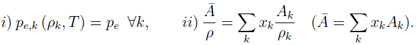
The disadvantages of the simple form of this new cold curve are on the one hand a lack of flexibility with only two free parameters. On the other hand sound speed is allowed to be discontinuous at the reference density.

Mixtures of elements

In the version of MPQeos I acquired the possibility for the calculation of mixtures of elements was not included. I added the so-called TF-mixing-of-elements method described in the QEOS description [4] to the FEOS library. The ionic contribution and the bonding correction are handled as a single species with mean atomic number Z and weight A. For the electronic contribution of the mixture the densities (effectively the partial volumes) of all species are iteratively adjusted in order to equilibrate all TF pressures and to fulfill an additive volume rule:

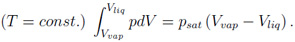
In these equations xk is the number fraction, and Ak is the atomic weight of species k.

The thermodynamic values for the electronic component of the mixture are finally obtained by summing up the single element values (with densities obtained by the above scheme), each weighted by xk Ak / A.

The described procedure is called for every density-temperature point, and therefore it is clear that the calculation of mixtures of elements is computationally more intensive than for a single element.

Calculation of liquid-vapor phase coexistence data

In the original MPQeos code the phase-coexistence data was calculated by the use of Maxwell's geometrical rule of equal areas below and above the van-der-Waals loop for each isotherm below the critical temperature:

Maxwell's rule is especially for low temperatures in the two-phase region computationally very intensive and imprecise. I solved this problem by adding a new routine for the coexistence data calculation. Now the coexistence boundary - also called the binodal - and the equilibrium or saturated vapor pressure are calculated with regard to the equilibrium of Gibbs' free energies and pressures on the liquid and the vapor side for each isotherm below the critical temperature. This leads to a large improvement of computational time and accuracy.

Example: Calculation of phase coexistence data for SiO2

Reference conditions and bulk modulus: Soft-sphere parameters:

Availability of the code

The code has been published together with the article [9] "The equation of state package FEOS for high energy density matter" in Computer Physics Communications:

Computer Physics Communications 227 (2018) 117–125, https://doi.org/10.1016/j.cpc.2018.01.008.

References

[1] S. Faik, An. Tauschwitz, J. Maruhn, I. Iosilevskiy; GSI Darmstadt; Report 2012-1, PNI-PP-12;

[2] T. Group; Report No. LALP-83-4, Los Alamos National Laboratory (1983);

[3] A. Kemp, J. Meyer-ter-Vehn, Nucl. Instrum. Methods A 415 (1998) 674;

[4] R. More, K. Warren, D. Young, G. Zimmerman; Phys. Fluids 31 (1988) 3059;

[5] S. Faik, M. Basko, An. Tauschwitz, I. Iosilevskiy, J. Maruhn; HEDP 8 (2012) 349-359;

[6] L. Thomas; Proc. Camb. Phil. Soc 23 (1927) 542; E. Fermi; Zeitschrift für Physik 48 (1928) 73;

[7] J. Barnes; Physical Review 153 (1967);

[8] D. Young, E.M. Corey; J. Appl. Phy. 6 (1995) 3748;

[9] S. Faik, An. Tauschwitz, I. Iosilevskiy; CPC 227 (2018) 117–125.